Linear Filter Estimation for Vision Neuroscience

A cell can be approximated as a temporal filter; that is, electrical input to the cell is processed, or filtered, and the output is different from the input as a result. The following notes explain the rationale behind treating cells as filters and highlight one standard method for mathematical filter extraction, white noise analysis. This particular method consists of inputting white noise to the cell (either directly e.g. by injecting current or indirectly e.g. by showing white noise visual stimulus to the organism) and then extracting the linear filter mathematically.

Introduction

Many different systems can be thought of as filters, and formal filter analysis/signals processing is used in many different fields. Some examples are audio processing and image processing; you might apply a low pass temporal filter to a noisy audio recording in order to remove “high frequency” background noise, and you might apply a “low pass” spatial filter to an image in order to soften, or blur it.

lowpass

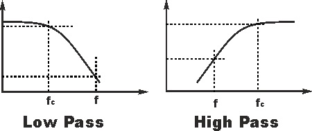
Low Pass and High Pass Filters in Frequency Space. The x-axis is frequency (Hz)

Low Pass High Pass

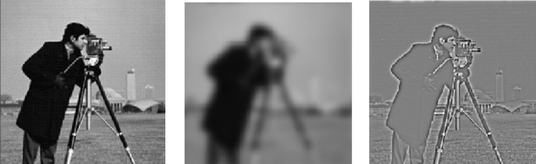
(Left) Original Image (Center) Image after applying a low pass filter (a.k.a blur) (Right) Image after applying a high pass filter (a.k.a sharpen)

Linear Filters

Linear systems have unique properties that allow for easy and powerful modeling and prediction. It is often incredibly helpful to approximate a physical system as linear, even if it isn’t “strictly” linear. Most signal processing techniques use this linear approximation because linear systems can be broken apart into smaller linear systems and then combined - this general principle is called linear superposition. What this means, for example, is that if we have 5 cells that are approximated as linear filters, we can extract the linear filter for each one and then combine them linearly to model/predict the overall response. This approximation is very helpful and has far reaching consequences. Thankfully, this can be done with many applications in science and engineering.

A system is strictly linear if it obeys two properties: homogeneity and additivity. Homogeneity means that an amplitude change in the input results in an identical amplitude change in the output (it is proportional). Additivity means that the sum of two input signals is equal to the sum of the respective output signals.

A good reference for digital signals processing is Smith, S. W. (1997). The scientist and engineer’s guide to digital signal processing. This can be accessed for free online at http://www.dspguide.com/

Static Nonlinearity

While many systems are completely linear (or linear within a certain regime), others are not. One way to get around this is to treat the system as Linear-Nonlinear (LN), which effectively means that you approximate the system as linear and then transform the linear prediction slightly to fit the experimental data with an instantaneous, i.e. “static,” nonlinearity. This approach is used quite frequently in vision neuroscience, and is described below.

Bussgang’s Theorem and White Noise Analysis

Unfortunately, once we start messing with nonlinearities (as in the LN model above), things can get complicated. With a purely linear system, we could design any kind of input stimulus and expect a linear a.k.a proportional output - for example, we could easily use sine wave gratings, images of trees, etc. as the input stimulus and expect a linear output. We could also extract the linear filter easily.

However, once we introduce something like a static nonlinearity, we have to be very careful with what type of stimulus input we use to extract the linear filter. Luckily, Bussgang’s theorem states the following:

The crosscorrelation of a Gaussian signal before and after it has passed through a nonlinear operation are equal up to a constant.

What this tells us essentially is that if we use Gaussian (white) noise as stimulus input, we can still extract a linear filter for our system despite having a nonlinearity. What this means in practice is that in order to extract a linear filter from a biological cell which we are approximating using the Linear-Nonlinear framework, we need the stimulus input to be Gaussian (white) noise.

Mathematically speaking, we have a model $r’=N(F*s)$ and the experimentally observed response $r$ and zero-mean stimulus $s$ (note the difference between model prediction $r’$ and experimental data $r$). We want to find the filter $F$ that best fits the model. On the assumption that the model is true (that $r$ is really generated as $N(F*s)$), Bussgang’s theorem allows us to find $F$ up to a constant of proportionality, regardless of the nonlinearity $N$, when $s$ is Gaussian. The theorem states, for $s$ a mean zero Gaussian with variance $\sigma^2$,

\begin{equation} \langle sN(Fs) \rangle= F {\langle ss \rangle} \langle \frac{d}{ds} N(Fs) \rangle \end{equation}

Substituting $r’=N(Fs)$ in the left side of the equation, this gives

\begin{equation} \frac{\langle r’s \rangle}{\langle ss \rangle} \propto F \end{equation}

(note that $\langle \frac{d}{ds} N(Fs) \rangle$ is just a constant). The left side of this equation is the expression for $F$ that results from a least-squares fit of the linear model $r’=Fs$ by linear regression. Note that the angled brackets here are defined as expectation, i.e. $ \langle x \rangle = \int x p(x) dx$ where $p(x)$ is the probability distribution of $x$.

White Noise Analysis for Temporal Filter

We finally arrive at the extraction of temporal linear filters. A linear filter is generally defined as:

\[response = Filter*stimulus\]

In some circumstances, we can simply divide the response by the stimulus in order to get the filter F:

\[Filter = response/stimulus\]

However, when dealing with temporal filters, the definition of a linear filter involves the mathematical operation of convolution:

\[r(t) = F(t) \circledast s(t)\]

If a fourier transform is applied, however, convolution becomes multiplication. Another way of saying this is that convolution becomes multiplication in Fourier space. We can therefore apply the Fourier transform and get multiplication:

\[\tilde{r}(\omega) = \tilde{F}(\omega) * \tilde{s}(\omega)\]

We therefore arrive at the method used in Baccus et al. 2002 and Behnia et al. 2014 (see the method sections of these papers). Linear filters in both of these papers were extracted by computing the following in Fourier space:

\[\tilde{F}(\omega) = \frac{\langle \tilde{r}(\omega) \tilde{s}(\omega) \rangle}{\langle \tilde{s}(\omega) \tilde{s}(\omega) \rangle} = \frac{\tilde{C}\_{rs}}{\tilde{C}_{ss}}\]

where $\tilde{C}_{rs}$ is the covariance between stimulus and response, and $\tilde{C}_{ss}$ is the autocovariance of the stimulus. Note that this uses Bussgang’s theorem, as above.

Filters in Vision Neuroscience

The following example from Baccus and Meister 2002 is particularly illustrative. In this study, they attempted to characterize the adaptive properties of the salamander retina to changing visual contrast. They recorded intracellularly from bipolar cells, amacrine cells and ganglion cells in the retina, and extracted filtering properties for each cell type based on the input stimulus. Among other things, they were able to show which cells adapted to contrast changes and which cells didn’t, based on their filtering analysis. The way they did this was straightforward - they extracted filters for each cell before and after the stimuli changed contrast, and compared them. Cells that adapted to contrast had different filters before and after, while cells that did not adapt to contrast had filters that remained the same.

The stimulus was a rapidly flickering uniform field whose light intensity changed randomly every 30 ms. They describe the method in the paper as follows:

The stimulus waveform $s(t)$ (i.e. the flickering light) is passed through a linear temporal filter $F(t)$
The result $g(t)$ is transformed by a static, nonlinear function $N(g)$ to the model’s response $r’(t)$
The filter $F(t)$ and the nonlinearity $N(g)$ are computed so the prediction of the model $r’(t)$ matches the measured neural response $r(t)$ as closely as possible

They explain:

Thus the linear filter summarizes the temporal processing between the stimulus and the neuron’s response, whereas the nonlinearity describes the instantaneous relationship between the filtered stimulus and the response. A intuitive description of the LN model is that the time reverse of the filter function $F(t)$ represents the stimulus feature to which the neuron is most sensitive. The filtered stimulus g(t) measures how strongly that feature is represented in the current stimulus, and the function $N(g)$ determines how $g(t)$ is transformed into a response, including the threshold effects, rectification, and other distortions.

baccusmeister

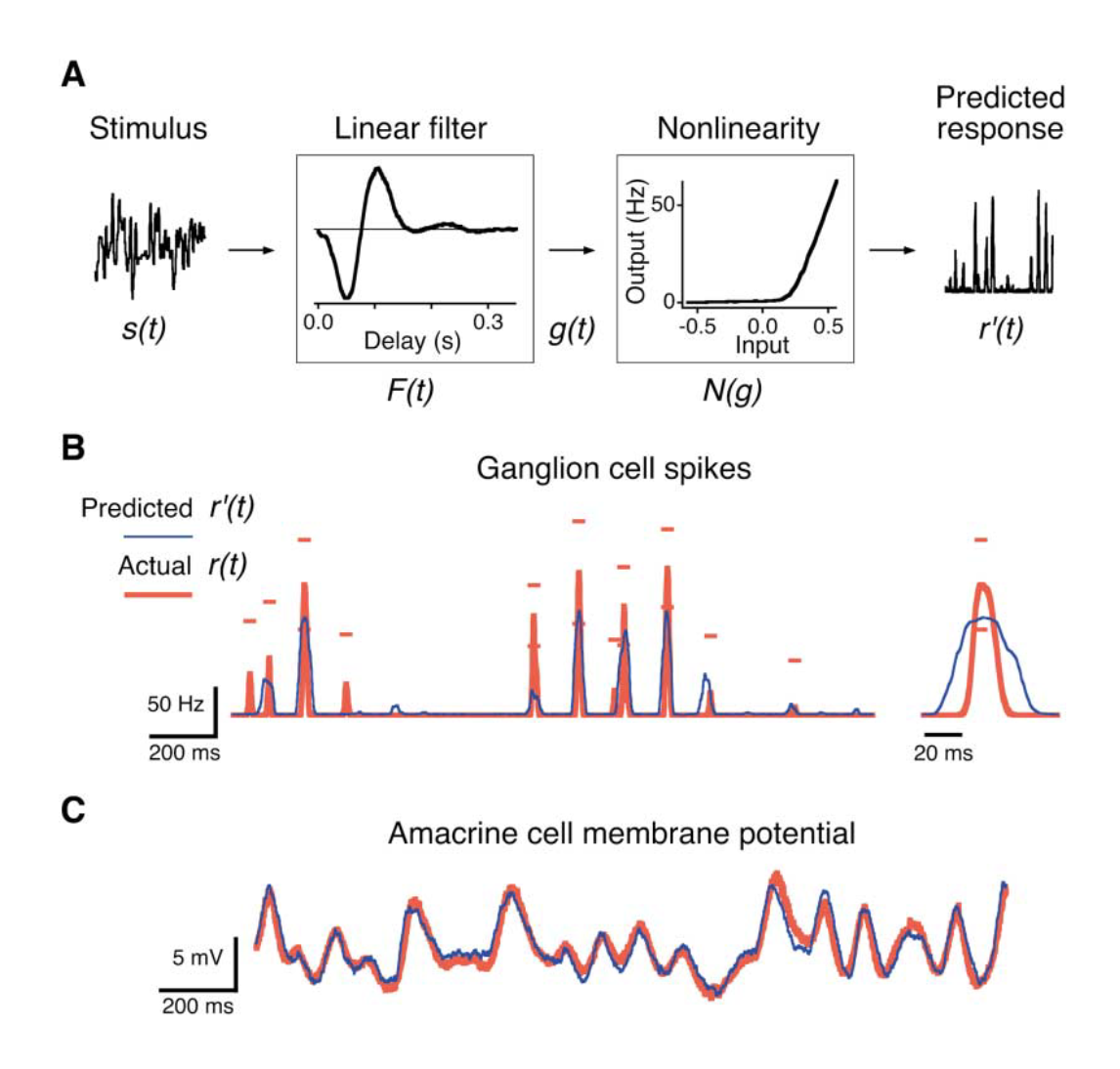
Image from Baccus et al. 2002 (Figure 2) (A) The Linear-Nonlinear (LN) model to predict the firing rate of a “fast OFF” ganglion cell. The flicker stimulus $s(t)$ is convolved with a linear filter $F(t)$, and then the result $g(t)$ is passed through a fixed nonlinearity $N(g)$ to produce the predicted firing rate $r’(t)$. (B) Predicted firing rate $r’(t)$ compared to the actual response $r(t)$. (C) The LN prediction of an amacrine cell membrane potential compared to the actual response. Segments displayed in (B) and (C) are representative of the entire recording.

References

Baccus, S. A., & Meister, M. (2002). Fast and slow contrast adaptation in retinal circuitry. Neuron, 36(5), 909-919.
Behnia, R., Clark, D. A., Carter, A. G., Clandinin, T. R., & Desplan, C. (2014). Processing properties of ON and OFF pathways for Drosophila motion detection. Nature, 512(7515), 427.
Chichilnisky, E. J. (2001). A simple white noise analysis of neuronal light responses. Network: Computation in Neural Systems, 12(2), 199-213.
Smith, S. W. (1997). The scientist and engineer’s guide to digital signal processing. http://www.dspguide.com/