Review of Transfer Functions for Linear Filters
Transfer functions sometimes come in handy when doing classical signals processing. These are some notes I took while working on questions of direction selectivity in the fly visual system.
Background: Transfer Functions and Bode Plots
Background: Helpful Mathematical Properties}
Some basic mathematical reminders:
*The magnitude of a complex number $ a + bi$ can be expressed as $ |a + bi| = \sqrt{a^2 + b^2}$
- The argument (phase) of a complex number $a + bi$ is $\phi = \arctan(\frac{b}{a})$
- $\arctan(x) = -\arctan(x)$ (remember that $\arctan(x)$ is the same as $\tan^{-1}(x)$)
- Finally, $\log(A/B) = \log(A) - \log(B)$ and $\log(A^2) = 2\log(A)$
I will use $i$ and $j$ interchangeably for the imaginary number
Note that $\arctan(0) = 0$ and $\arctan(-x) = -\arctan(x)$.
Phase of a complex number $ z = a + j \omega$
\begin{equation} \angle z = \arctan(\omega/a) \end{equation}
Gain is often plotted as $\log_{10}(|G(j\omega)|)$
$360^{\circ} = 2 \pi$ radians, so $1^{\circ} = \pi/180$ radians and 1 radian $= 180/\pi = 57.29577 ^{\circ}$
Here is a quick reference on transfer functions: https://web.njit.edu/~levkov/classes_files/ECE232/Handouts/Frequency\%20Response.pdf
Example 1
The transfer function of
\[f(t) = e^{-t}\]is
\[H(s) = \frac{1}{s+1}\]The magnitude of the transfer function is given by:
\[|H(s)| = \frac{1}{\sqrt{(\omega^2 + 1)}}\]In order to calculate the phase, we can rearrange the transfer function into $\Re$ and $\Im$ components:
\[H(s) = \frac{a}{s+a} \longrightarrow \frac{a}{a+ j\omega} \cdot \frac{a - j \omega}{ a- j \omega} = \frac{a^2 - j a \omega}{a^2 - j^2 \omega^2} = \frac{a^2}{a^2 + \omega^2} - \frac{a \omega}{a^2 + \omega^2} j\] \[\angle H(s) = \phi = \arctan\Big( \frac{-a\omega}{a^2} \Big) = \arctan\Big( \frac{-\omega}{a} \Big)\]converting this to degrees we have
\[\angle H(s) = \phi = -\frac{180}{\pi} \arctan\Big(\frac{\omega}{a}\Big)\]A simpler way of calculating this is by using the straightforward rules (that are the result of carrying the phase in the exponential)
\begin{equation} \angle [G_1(s)\cdot G_2(s)] = \angle [G_1(s)] + \angle [G_2(s)] \end{equation}
\begin{equation} \angle [G_1(s)/G_2(s)] = \angle [G_1(s)] - \angle [G_2(s)] \end{equation}
We then get
\[\angle H(s) = \angle [\frac{a}{s+a}] = \angle a - \angle[j \omega +a] = \arctan(0) - \arctan\Big(\frac{\omega}{a}\Big)\]Example 2
The Laplace transform of
\[f(t) = a \cdot e^{-at}\]is
\[H(s) = \frac{a}{(s+a)}\]The magnitude of the transfer function is given by:
\[= \log|a| - \log|j\omega + a| \rightarrow \log(a) - \log( \sqrt{\omega^2 + a^2} ) \rightarrow \log(a/\sqrt{\omega^2 + a^2})\] \[|H(s)| = \frac{a}{\sqrt{\omega^2 + a^2}}\]The phase remains the same as before, since their is no phase contribution due to the numerator $a$
\[\angle H(s) = - \arctan\Big(\frac{\omega}{a}\Big)\]Example 3
Low Pass Filters $ f(t) = a t \cdot e^{-at} $ and $ f(t) = a^2 t \cdot e^{-at} $
For $ f(t) = a t \cdot e^{-at} $, the transfer function is
\[H(s) = \frac{a}{(s+a)^2}\]and the magnitude is
\[\|H(s)\| = \frac{a}{(\omega^2 + a^2)}\]However, this does not seem to normalize the response, so there is a simple gain effect at low frequencies from the amplitude itself. We can normalize the gain by taking $\omega \rightarrow 0$ and fixing $|H(s)| = 1$:
\[f(t) = a^2 t \cdot e^{-at} \rightarrow |H(s)| = \frac{a^2}{(\omega^2 + a^2)}\]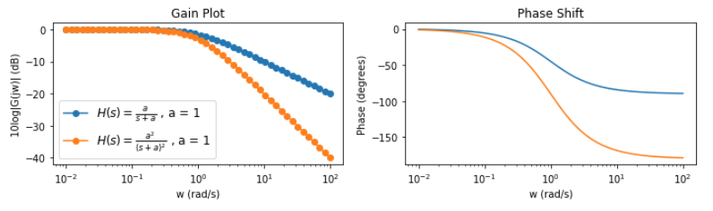
Comparison of Gain and Phase for two versions of filters. An important detail is that the filter $f(t)=a^2te^{-at}$ has a phase shift from $0$ to $180^\circ$
The phase for both of these are is:
\[\angle \Big[ \frac{a}{(s+a)^2} \Big] \longrightarrow \frac{a^3 - a\omega^2}{(a^2 + \omega^2)^2} - j\frac{2a^2\omega}{(a^2 + \omega^2)^2} \longrightarrow \arctan\Big( \frac{-2a^2\omega}{a^3 - a\omega^2} \Big)\] \[\angle \Big[ \frac{a^2}{(s+a)^2} \Big] \longrightarrow \frac{a^4 - a^2\omega^2}{(a^2 + \omega^2)^2} - j\frac{2a^3\omega}{(a^2 + \omega^2)^2} \longrightarrow \arctan\Big( \frac{-2a^3\omega}{a^4 - a^2 \omega^2} \Big)\]