Velocity Estimation via Derivatives
How might a biological system estimate velocity?
Chapter 8 of the book Visual Perception: Physiology, Psychology and Ecology by Bruce, Green and Georgeson contains a wealth of information about image-based computation of motion. These notes are taken directly from this chapter.
Movement is a change of position over time.The change in position divided by the time taken gives the velocity of movement. This simple intuition forms the basis for a class of models of motion perception known as correspondence models, since with this approach the major problem is that of matching things over time.
Our aim is to show how motion information can in principle be recovered from the space-time image, and then to show that the various models form a single family, differing not so much in principle but in implementation.
\begin{equation} x - v \cdot t = x_i \end{equation}
A complete description of the moving pattern is given by its space time image $I(x,t)$. Intuitively, the tilt of the space0time image away from the vertical gives the speed of motion - another way to say this is that motion is orientation in space time. A basic task in motion perception is to recover the velocity $v$ from the time-varying retinal input, and this can be seen a the task of recovering the orientation of the space-time image.
Velocity as a function of spatial and temporal derivatives
The intensity of an image moving at constant velocity $v$ at any point $x$ and time $t$ is some function $I(x-v \cdot t)$
\begin{equation}\label{eqn: Ix} \frac{\partial I}{\partial x} = I’(x-vt) \end{equation}
\begin{equation}\label{eqn: It} \frac{\partial I}{\partial x} = -v \cdot I’(x-vt) \end{equation}
Combining these two equations we get: \begin{equation} \frac{\partial I}{\partial t} = -v \cdot \frac{\partial I}{\partial x} \end{equation}
which leads us to:
\begin{equation} \label{eqn: v} v = -\frac{\partial I /\partial t}{\partial I /\partial x} \end{equation}
Another way to derive this:
- Pixel intensities of an object do not change between consecutive frames
- Neighbouring pixels have similar motion
The under-constrained “Optical Flow equation” can be derived as follows. The above assumptions imply that: \begin{equation} I(x,t) \approx I(x+\Delta x, t + \Delta t) \end{equation} Making a Taylor series approximation and taking the first order terms \begin{equation} I(x+\Delta x,t+\Delta t) = I(x,t) + \frac{\partial I}{\partial x}\Delta x+\frac{\partial I}{\partial t}\Delta t \end{equation} By assuming that the pixel intensity $I$ remains constant during the short time interval $\Delta t$, we can simplify the equation to: \begin{equation} \frac{\partial I}{\partial x} \Delta x + \frac{\partial I}{\partial t} \Delta t = 0 \end{equation}
\begin{equation} \frac{\partial I}{\partial x} \frac{\Delta x}{\Delta t} + \frac{\partial I}{\partial t} = 0 \end{equation}
This finally leads to: \begin{equation} \frac{\partial I}{\partial x} v + \frac{\partial I}{\partial t} = 0 \end{equation}
\begin{equation} v = - \frac{\partial I /\partial t}{\partial I /\partial x} \end{equation}
Multi-channel gradient model: Encoding velocity via 1st and 2nd derivatives
Let $ I_x = \partial I / \partial x$, $I_{xx} = \partial I /\partial x \partial x$ and $I_{xt}=\partial I / \partial x \partial t$. Differentiating equation \ref{eqn: v} with respect to $x$ gives:
\begin{equation} \label{eqn: Ixt} I_{xt} = -v \cdot I_{xx} \end{equation}
Multiplying equation \ref{eqn: It} by $I_x$ and equation \ref{eqn: Ixt} by $I_{xx}$ gives:
\begin{equation} I_x I_t = -v \cdot I_x I_x \end{equation}
\begin{equation} I_{xx} I_{xt} = -v \cdot I_{xx} I_{xx} \end{equation}
Adding these two equations with a weighting factor $w^2$ gives:
\begin{equation}
v = - \frac{(I_x I_t + w^2 I_{xx}I_{xt})}{(I_x^2 + w^2 I_{xx})}
\end{equation}
This is more robust than equation \ref{eqn: v}, since $I_x$ and $I_xx$ are not usually zero-valued simultaneously.
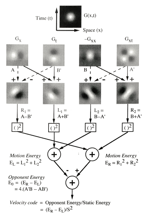
Motion-Energy model with spatiotemporal filters chosen as first and second order gaussian derivatives. This is from Figure 8.8 in Visual Perception (page 224)
Velocity from Motion-Energy
$R_1 = A-B’$ $L_1 = A+B’$ $L_2 = B-A’$ $R_2 = B+A’$. These are the filters that are oriented in space-time. Applying a squared nonlinearity to each and summing pairs gives the left and right motion-energy:
\(E_L = L_1^2 + L_2^2\) \(E_R = R_1^2 + R_2^2\)
Subtracting $E_L$ from $E_R$ gives the opponent energy:
\(E_O = E_R - E_L\) \(= R_1^2 + R_2^2 - (L_1^2 + L_2^2)\) \(= (A-B')^2 + (B+A')^2 - (A+B')^2 - (B-A')^2\) $= A^2 + B^2 -2AB’ + B^2 + A’^2 + 2A’B -(A^2 + B’^2 + 2AB’) - (B^2 + A’2 - 2A’B)$
\begin{equation} E_O = 4(A’B - AB’) \end{equation}
It is important to note that opponent energy does not estimate velocity, in part because it varies with contrast (how?)
Adelson and Bergen (1985) noted that a veridical velocity estimation could be recovered if the opponent energy signal was divided by a “static energy” signal, AND the filters $A$,$B’$, $A’$ and $B$ are chosen carefully.
Since $A$ and $B$ are nondirectional spatial filters with the same temporal response but are $90\deg$ out of phase spatially, the static energy might be something like:
\begin{equation} S^2 = 4 (A^2 + B^2) \end{equation}
Thus the velocity estimate is:
\begin{equation} v = E_O/S^2 = \frac{(A’B - AB’)}{(A^2 + B^2)} \end{equation}
How does this relate to the velocity estimate above based on first and second order derivatives?
The similarities are striking
\begin{equation} v = \frac{(A’B - AB’)}{(A^2 + B^2)}, \space v = - \frac{(I_x I_t + w^2 I_{xx}I_{xt})}{(I_x^2 + w^2 I_{xx})} \end{equation}
These two estimates of velocity are equivalent if we let $A=I_x$, a first order derivative in space, $A’ = wI_{xt}$, the outer product of a first order derivative in space and a first order derivative in time, $B=-wI_{xx}$, a second-derivative in space, and $B’=I_t$, a first order temporal derivative.
Relationship to Optical Flow Algorithms
Optical flow estimates can be used to determine structure from motion and has applications in video compression and video stabilization. The underlying assumptions are that
- Pixel intensities of an object do not change between consecutive frames
- Neighbouring pixels have similar motion
The under-constrained “Optical Flow equation” can be derived as follows. The above assumptions imply that: \begin{equation} I(x,y,t) \approx I(x+\Delta x,y + \Delta y , t + \Delta t) \end{equation} Making a Taylor series approximation and taking the first order terms \begin{equation} I(x+\Delta x,y+\Delta y,t+\Delta t) = I(x,y,t) + \frac{\partial I}{\partial x}\Delta x+\frac{\partial I}{\partial y}\Delta y+\frac{\partial I}{\partial t}\Delta t \end{equation}
\begin{equation} \frac{\partial I}{\partial x} \Delta x + \frac{\partial I}{\partial y} \Delta y + \frac{\partial I}{\partial t} \Delta t = 0 \end{equation}
\begin{equation} \frac{\partial I}{\partial x} \frac{\Delta x}{\Delta t} + \frac{\partial I}{\partial y} \frac{\Delta y}{\Delta t} + \frac{\partial I}{\partial t} = 0 \end{equation}
This finally leads to: \begin{equation} \frac{\partial I}{\partial x} V_x + \frac{\partial I}{\partial y} V_y + \frac{\partial I}{\partial t} = 0 \end{equation} where $V_x$ and $V_y$ are the velocity components and the derivatives are the derivatives of the image for the spatial and temporal components. This can be rewritten as: \begin{equation} \nabla I^T\cdot\vec{V} = -I_t \end{equation}
This equation cannot be solved without additional constraints; this is known as the aperture problem. Variational, differential algorithms such as Lucas-Kanade and Horn-Schunk impose additional constraints by assuming that the displacement of the image contents between two nearby frames is small and approximately constant within a neighborhood of the point p under consideration.
References
-
Adelson, Edward H., and James R. Bergen. Spatiotemporal energy models for the perception of motion. Josa a 2.2 (1985): 284-299.
-
Bruce, Vicki, Patrick R. Green, and Mark A. Georgeson. Visual perception: Physiology, psychology, & ecology. Psychology Press, 2003.